Pollutant Emission Rate Calculation

Introduction

Process measurement usually requires hardware sensors to convert process variables to electronic signals for processing and transmitting. Soft sensors refer to indirect methods that use analytical calculation to derive required process variables. When hardware sensors are not available or difficult to obtain in real time, soft sensors provide an alternative for monitoring or control. In this article, two soft-sensor use cases are discussed to demonstrate this method and its benefits.

Emission Rate Calculation

Pollutant emission rate in industrial fired units need to meet stringent regulatory requirement due to environmental concerns. The interested variables are the mass flow rate of pollutant, such as SO2 in the unit of gram per second (g/s). However, many decades-old units lack flue gas flow measurement to provide pollutant flow rate. Instead of installing specialized flue gas flow rate measuring instrument, an alternative approach is to calculate pollutant flow rate based on combustion balance equation and available instruments.

In a fired unit, the following measurements are usually available for combustion control purpose: fuel gas flow rate, flue gas excess oxygen content, and pollutant emission in PPM (parts per million). Air flow rate is measured when it is being modulated; for natural draft units, however, air flow is often not measured.

Here we consider a natural draft fired unit that uses natural gas (methane) as fuel gas and need to calculate its pollutant emission rate. Following measurement is available:

1. Fuel gas flow rate F
2. Fuel gas density D
3. Flue gas oxygen content in percentage e%
4. Pollutant content in flue gas x PPM

We are looking for pollutant mass flow rate y in g/s. Assume x PPM is the mass ratio between pollutant and flue gas. It follows then we just need to calculate the mass flow rate of flue gas. As we have only fuel gas flow mass flow rate, we will need air flow rate or excess air ratio to obtain the flue gas flow rate.

Based on methane combustion equation with k% excess air:

$$\text{CH}_4 + 2(1+k\%)\text{O}_2 + 2(1+k\%)\times 3.76\,\text{N}_2 \rightarrow \text{CO}_2 + 2\text{H}_2\text{O} + 2k\%\,\text{O}_2 + 2(1+k\%)\times 3.76\,\text{N}_2$$

Assume all water product stays in vapor state in flue gas. The mass ratio of excess oxygen in the flue gas can be obtained based on molecular weight of each component and the excess air ratio:

$$e\% = \frac{2k\% \times 32}{44 + 36 + 2k\% \times 32 + 2(1+k\%) \times 3.76 \times 28}$$

Re-arranging above equation gives:

$$k\% = \frac{290.56 \times e\%}{64 - 274.56 \times e\%}$$

This provides excess air ratio based on oxygen measurement in flue gas.

Combined with other three measurements, F, D, and x, the pollutant mass flow rate can be calculated as:

$$Y = x \times \frac{F}{D} \times \frac{44 + 36 + 2k\% \times 32 + 2(1+k\%) \times 3.76 \times 28}{1{,}000{,}000}$$

Note this equation provides pollutant flow rate in the same unit as the fuel gas flow rate. Unit conversion factors may need to be applied to obtain pollutant flow rate in g/s.

This method was applied to actual data in a fired heater and calculation results are listed below:

1. Fuel gas flow rate: F = 120.16 MCF/H (thousand cubic feet per hour)
2. Fuel gas density: 0.231 lb/CF (pounds per cubic foot)
3. Flue gas oxygen content e% = 5.80786%
4. Pollutant content x = 20.11 PPM
5. Calculated excess air ratio k% = 0.351
6. Calculated fuel gas flow rate is 63834.42 g/s
7. Calculated pollutant flow rate is 1.284 g/s

Although there is no flue gas mass flow instrument available to cross check results, the calculation is based on well-established combustion equation and the result is in the expected order of magnitude. Therefore, this soft-sensor based method can be used for emission rate monitoring.

Disturbance Reduction

Disturbance is the enemy of a control system. It is an unwanted variable that can cause deviation of controlled variable from desired setpoint; its effects must be minimized. If disturbance can be measured and its dynamic model is known, a feedforward action can be added to controller output or Manipulative Variable (MV) to cancel out its effect on Controlled Variable (CV). However, most disturbance variables in practice are unknown and not measured. Controller cannot deal with unknown variables; only when disturbance starts affecting CV, controller can calculate deviation error and adjust MV to restore CV back to its setpoint. This is the advantage of a feedback loop: It can counter any disturbance inside the loop. But it needs to see deviation before control action can be applied, a limitation of a feedback loop.

If soft sensor can provide virtual measurement of disturbance, an estimate calculated based on analytical relationships between the disturbance variable, unknown disturbance becomes available for feedforward control and the effects of disturbance can be compensated before causing deviation to controlled variable. This method can improve control performance without adding extra hardware sensor measurement.

For example, consider a dryer process as shown in the figure below.

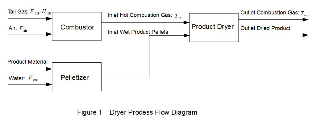
Product material is made into wet pellets by adding water in pelletizer. Once pellets are formed, water and moisture are removed by a dryer, a heat exchanger where hot combustion gas generated from combustor heats up and dries pellets. Combustor burns a waste product, tail gas, generated from production process. As product grade changes, the heating value of tail gas also varies.

Key process variables are shown in above diagram. FTG and HTG are the flow rate and heating value of tail gas; FTG is the combustion air flow rate; Fwtr is the water flow rate to the pelletizer; Tin and Tout are the inlet and outlet temperatures of the hot combustion gas temperature.

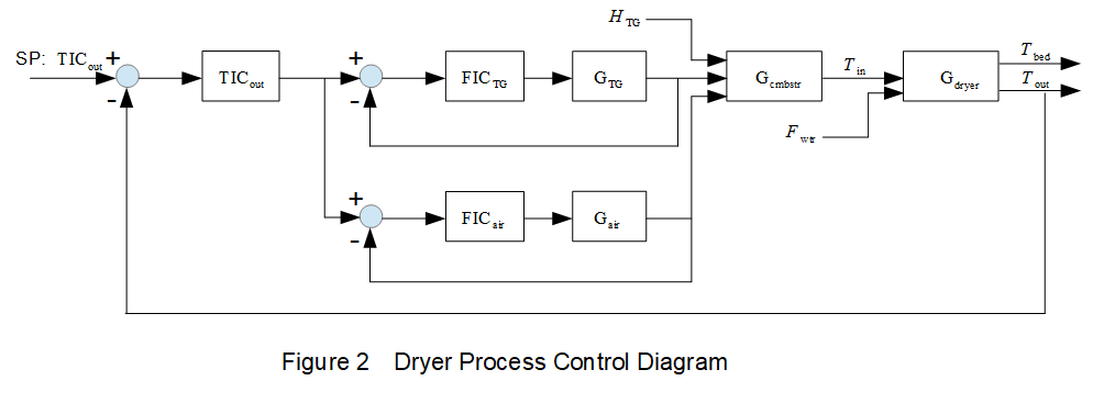
In the diagram, TIC represents the temperature indicating controller, FIC represents flow indicating controller, G represents the transfer function between input and output. The subscripts are the acronyms of variables or equipment, such as outlet temperature, tail gas flow, combustor, dryer, etc. The diagram shows the connections of multiple single variable PID feedback control loops. The dryer outlet temperature control TICOUT is the master PID controller. Its control output is sent to the flow controllers of tail gas and combustion air. Note these two flow controllers are part of combustion control and have cross limiting setup to ensure air increases before tail gas flow and decreases after tail gas flow. The tail gas flow, combustion air flow, and tail gas heating value are inputs of the combustion process and determine dryer inlet temperature Tin. This inlet temperature and the water flow are the inputs to the dryer process and determine dryer outlet temperature and bed temperature, taken from the dryer product side.

This process is to remove the moisture in product pellets by using tail gas combustor and dryer. Moisture measurement is difficult and expensive to implement; therefore, temperature is used to indicate the effect of moisture removal. The PID control loops are designed around dryer outlet temperature, because its response time to a combustion and pelletizer water flow change is shorter. The product temperature of the dryer beds is better indication for moisture removal, but its response time is much longer because of additional heat transfer process between combustion gas and product pellets. On a setpoint change of dryer outlet temperature, outlet temperature settles in about 20 to 40 minutes, while bed temperature settles in 100 to 180 minutes.

Bed temperatures are also affected by pelletizer water flow and tail gas heating value. Because of the slow response and multiple variable features of the process, it is difficult to set up another PID loop to control bed temperature by adjusting outlet temperature loop setpoint. Operator can manually adjust it by experience but need to keep track data in the past 2 to 3 hours. This is a best application case for advanced multi-variable control such as Dynamic Matrix Control (DMC).

DMC Implementation

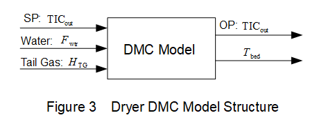
The following diagram shows the typical input/output model structure. The CVs are shown on the output side of model: controller output of TICOUT and process variable bed temperature. Controller output is included to avoid DMC saturating PID control loop. The setpoint of TICOUT is MV and DMC adjusts it to achieve desired targets of CV; water flow and heating value are Disturbance Variables (DV) and DMC monitor them and adjust MV to cancel out their effects on CV.

There is one difficulty implementing above control structure: The heating value is typically obtained by combustion analysis of the fuel gas and not available for real-time control. Apparently, when not measured, even advanced control like DMC cannot use it for feedforward control. For example, if there is a product grade change and the heating value of tail gas increases, combustor will generate more heat under same tail gas and air flow rates; consequently, dryer inlet, outlet, and bed temperatures will all increase. Outlet PID loop will reduce control output and DMC will reduce MV, the setpoint of outlet temperature loop, which further reduces loop control output. For a slow temperature control loop, this feedback compensation action only slowly compensates the deviation caused by unknown disturbance. Although feedback compensation can eventually bring temperature back to setpoint, it often leads to oscillations.

The above scenario is known to operators and engineers at plant. As heating value most often changes during product grade change, operator is asked to turn off DMC and manually adjust outlet temperature control setpoint to control dryer bed temperature. This is not an ideal situation, but there was not a solution for an unknown disturbance until a soft sensor method was recently established. The idea is to calculate heating value change in the unit of mega-joules per nominal cubic meter (MJ/NM³), based on known product grade and other process conditions. The method is similar to emission rate calculation discussed in previous section.

Results

With heating value available as a quantitative process variable, it becomes possible to model its effects on bed temperatures and include it in DMC.

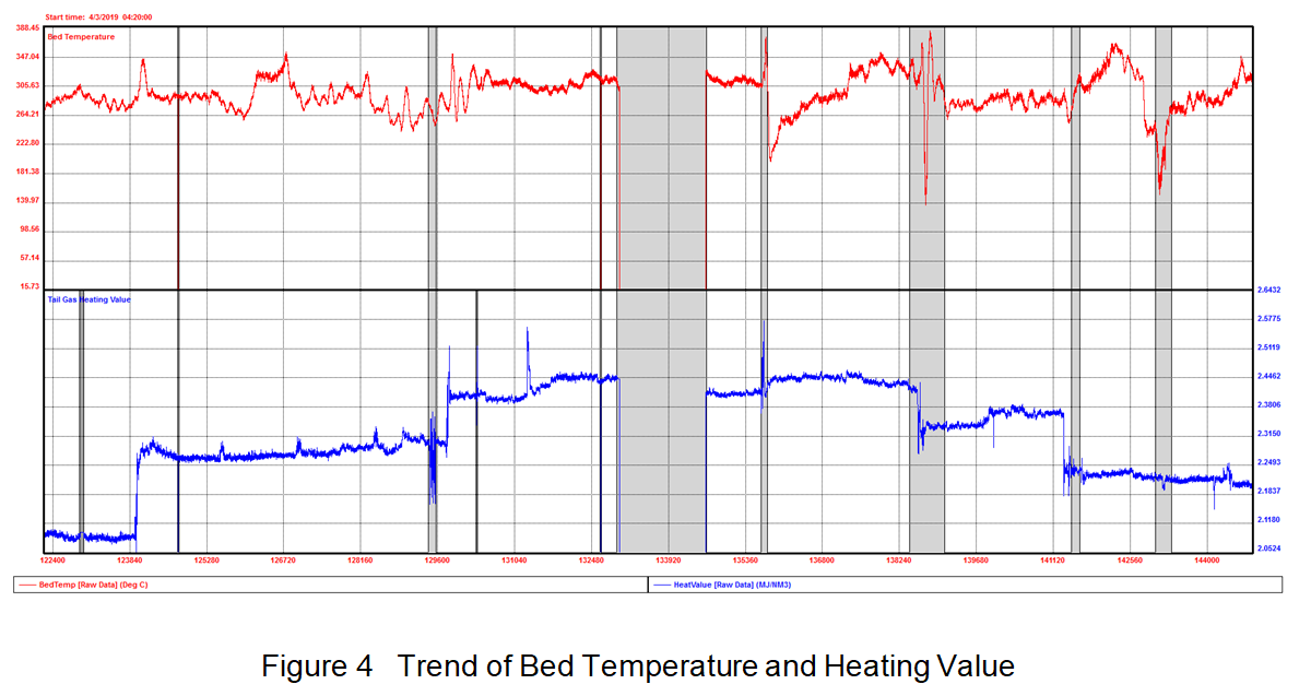
For example, in the figure below, the red line is the data for bed temperature and blue line for heating value. Bed temperature has clearly frequent temperature spikes and these abrupt changes appear to be correlated with heating value changes.

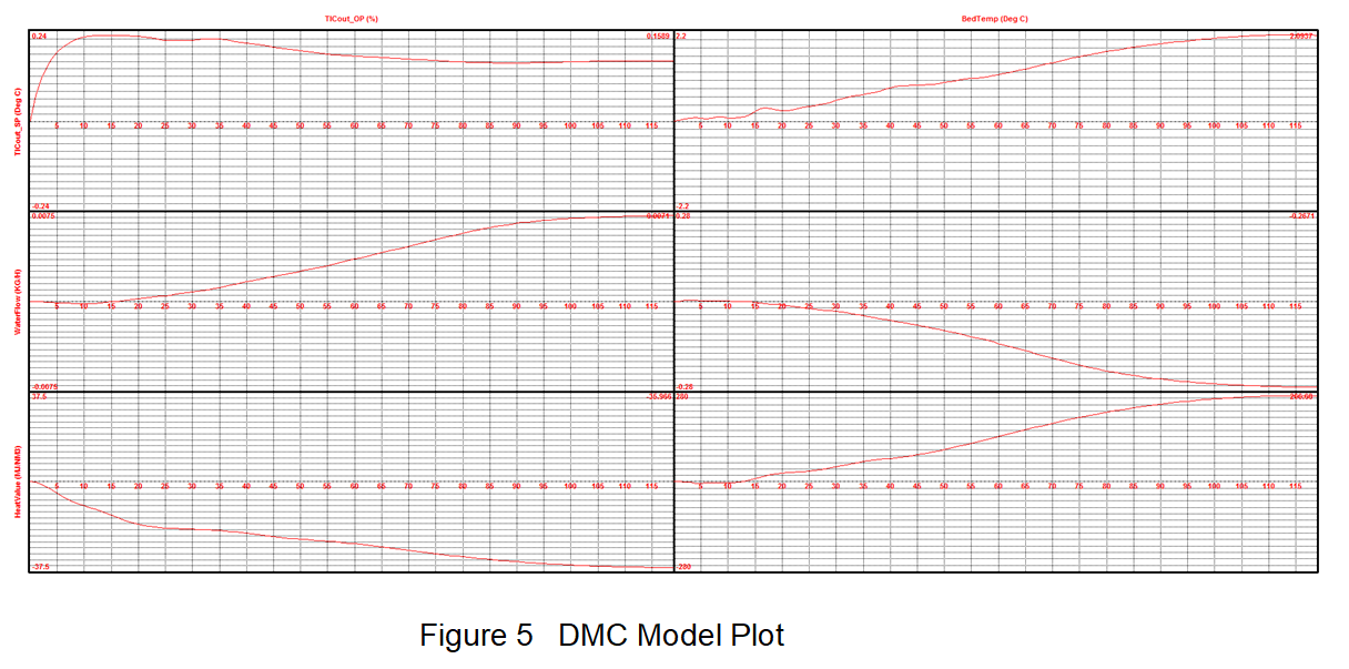
After feeding this historical data into DMC modeling tool, the response curves were identified. As there are three inputs (one MV, two disturbance variables) and two CVs, the curves are arranged in a 3-by-2 array. The bed temperature responses are shown in the second column. From top to bottom, the three inputs are outlet temperature controller setpoint, water flow, and heating value. The curve shows a first-order response between bed temperature (CV) and input variables. The responses all have settling time of about 120 minutes, but with significantly different steady-state gains: 2.2, -0.28, and 280. These gains indicate the bed temperature change in steady state when input variable has a step change. For example, if heating value increases by 1 MJ/NM³, the bed temperature will increase by 280°C in steady state. In comparison, bed temperature changes by 2.2 and -0.28 upon changes by outlet temperature controller setpoint and water flow. Even with consideration of unit difference, the heating value still has most significant impact on bed temperature. Therefore, it is not surprising to observe bed temperature deviation due to heating value changes.

The figure below shows the data of bed temperature before and after DMC is turned on for bed temperature control. Before the first gray bar, operator was manually adjusting outlet temperature controller. Apparently, the amplitude of bed temperature deviation is reduced by more than half when DMC starts control. Moreover, the second gray bar shows: when heating value decreased by 0.2 MJ/NM³, there was no deviation observed on bed temperature. The effects of heating value disturbance has been predicted and compensated in advance by controller. This is a feedforward action and has fully eliminated disturbance effect. Operation and engineers were very happy with the control performance. Now product grade change can be handled by DMC with no noticeable effects on bed temperature.

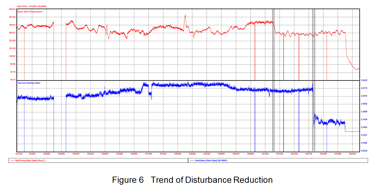
A couple of side notes on the trend: 1) bed temperature dropped when DMC turned on because operation reduced bed temperature setpoint; 2) bed temperature dropped to flat line at the end of trend because dryer was shut down for maintenance.

Summary

This article discussed two application examples when soft sensor can become particularly useful:

1. For measurement where dedicated hardware sensors were not installed but analytical calculation can be applied based on other existing sensors.
2. In multi-variable control application where key disturbance variable cannot be measured in real-time by hardware sensors, but the disturbance cannot be reduced by feedback controllers. Feedforward control action can be applied to eliminate disturbance when soft sensor provides virtual measurement and disturbance model is identified from historical data.