Practical Frequency Domain Concepts
Practical Frequency Domain Concepts
Introduction: Why Frequency Thinking Matters — Even Without Models
Frequency domain method is taught in every control textbook. But in practice, many engineers avoid frequency domain methods because they believe they need complex software and perfect mathematical models. However, the core insights from frequency domain analysis can be applied using simple, practical approaches. Plus, readily available open source packages such as the Python Control library can provide sufficient tools for this analysis.
The core insight of frequency domain analysis lies in recognizing that different controller performance requirements dominate specific frequency regions.
Frequency-Domain Separation of System Requirements
Low-Frequency Region
- Control Objective: Steady-state accuracy and disturbance rejection
- Signal Content: Command signals and low-frequency disturbances
- Controller Requirement: High gain to minimize steady-state errors
- Mathematical Basis: Final Value Theorem dictates that high low-frequency gain ensures excellent reference tracking and disturbance attenuation
Mid-Frequency Region
- Control Objective: Stability, robustness, and transient response
- Signal Content: System’s natural dynamics and control bandwidth
- Controller Requirement: Appropriate phase/gain margins for stability
- Mathematical Basis: Gain/phase margins at crossover frequency determine damping and overshoot characteristics
High-Frequency Region
- Control Objective: Noise immunity and robustness to unmodeled dynamics
- Signal Content: Sensor noise and high-frequency disturbances
- Controller Requirement: Attenuation to prevent noise amplification
- Mathematical Basis: Roll-off characteristics protect against high-frequency uncertainties
This frequency-based separation allows engineers to design controllers that optimize performance where it matters most, while maintaining robustness against uncertainties and disturbances. For standard PID controllers, tuning the controller parameters can have direct effect on shaping the frequency response plots.
Worked Example: FOLPD Process
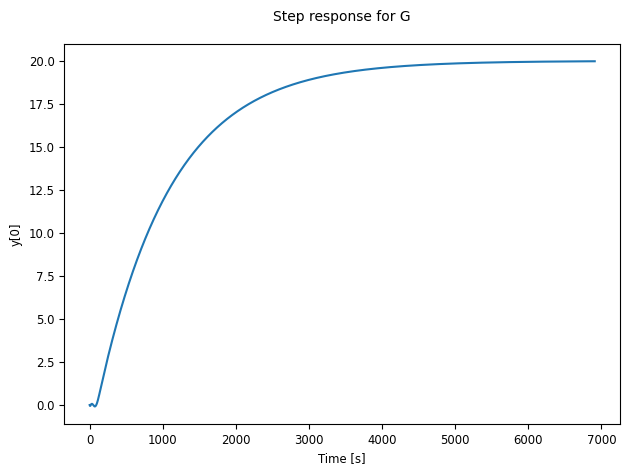
Now, let’s see one example. Suppose we have a process that is first-order lag with pure time delay. The time constant is 1000 seconds, delay is 100 seconds, and static gain is 20, which leads to a slow step response as shown below. It takes about 3000 seconds to approach the final value.
Its Bode plot of frequency response is shown as follows:
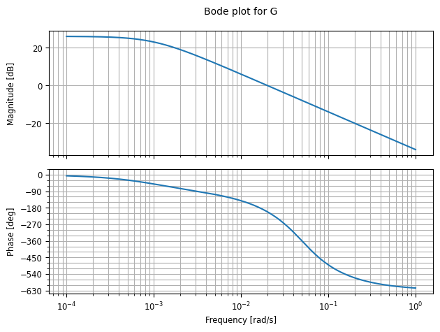
Here we can see the magnitude at lower frequency range is about 25 dB, and it decreases at about 20 dB per decade. The magnitude starts decreasing at about 0.001 rad/s, which agrees with the time constant of 1000 seconds. These are the typical characteristics of a first-order lag process. The phase plot shows a combination of lag process and time delay. Standard first-order lag process has maximum -90 degrees phase; with time delay of 100s, it reaches -180 degrees at about 0.015 rad/s. Note at the frequency 1/100 = 0.01 rad/s, the phase is about -135 degrees. This is a critical frequency that limits the system performance.
Adding a PI Controller
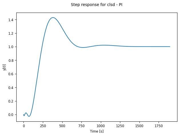
Now, let’s use a typical Proportional and Integral (PI) controller to improve its response. When selecting the integration period as 300 seconds, and proportional gain as 0.375, the step response becomes much faster but with high overshoot.
The Bode plot of this PI controller is shown below.
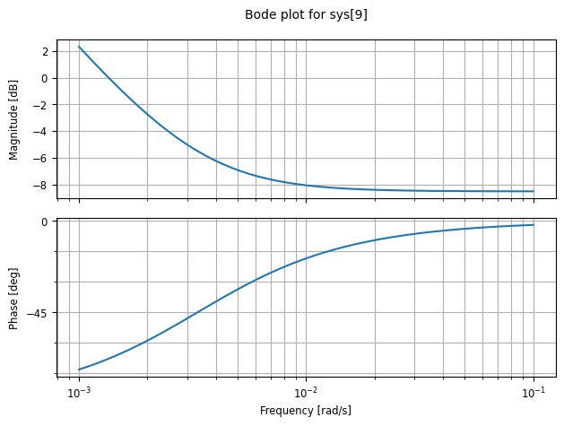
Notice the PI controller has higher gain and phase lag at low frequency. The gain and phase lag diminish at high frequency. This PI controller has modified the frequency response of the process as shown in the following Bode plot of the loop transfer function.
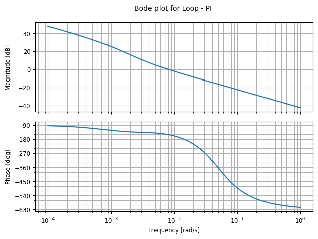
Notice this response has gain crossover frequency of around 0.008, which shows a higher bandwidth than the original process. At this frequency, the phase lag is less than 180 degrees, but the difference is only about 22.5 degrees. In other words, its phase margin is very small. Systems with small phase margin will have response curves with high overshoot. Intuitively, when phase margin reduces to 0, the response will have sustained oscillations.
Adding Derivative Action: PI → PID
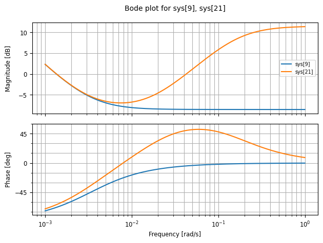
To reduce overshoot and improve phase margin, we could add a derivative action of 60s to the PI controller. The following is a Bode plot of a PID controller (orange curve) compared with the previous PI controller (blue curve). The derivative action adds phase lead between roughly 0.01 to 0.1 rad/s.
The Bode plots of the two loop transfer functions are shown below:
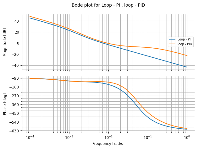
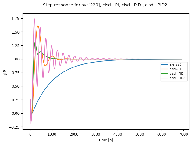
Notice the PID loop has similar crossover frequency around 0.008, but the phase margin has been increased to about 60 degrees. High phase margin means the system has high damping and lower overshoot, as shown in the following step response comparisons.
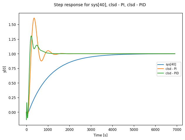
Note the original step response has been adjusted to static gain of 1 to put all curves on the same scale. Clearly, the PID provides similar fast response as the PI controller but with smaller overshoot.
Pushing Further: The Dead-Time Limit
Now we have seen that higher crossover frequency (bandwidth) increases response speed, and higher phase margin reduces overshoot. Though the above response looks much better, you may want to see if it can be improved further by increasing the crossover frequency while maintaining similar phase margin for small overshoot.
Following PID2 controller uses a slightly higher gain and higher derivative time, which increases gain crossover frequency while maintaining similar phase curves, as shown in Bode plots below.
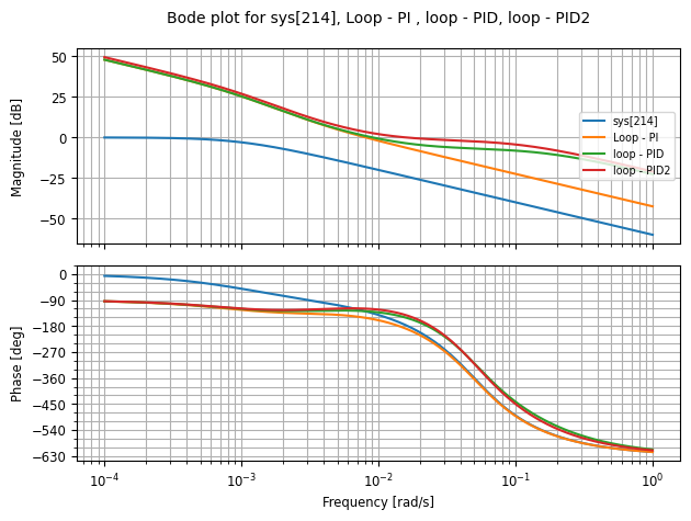
However, because of the time delay in the process, the phase lag increases with frequency and the phase margin of this PID2 is less than 20 degrees. As a result, its response curve is oscillating.
This confirms the previously mentioned critical frequency around 1/100 = 0.01 rad/s. Because of time delay at 100s, the gain crossover frequency needs to be less than this limit to allow for good phase margin. Only when the time delay constant is reduced, this limit will prevent further improvement of response.
With this example, I hope you have seen how three frequency concepts and simple plotting tools can guide in understanding and tuning controllers in practice.
The Three Practical Frequency Concepts
1) System Bandwidth — The “Speed Control Knob”
What it is: The frequency range where your system can effectively respond to changes.
Practical Estimation:
- Step response rise time ≈ 2.2 / Bandwidth
PID Connection: Increasing Kp raises bandwidth → faster response
Simple Rule: If you want 2× faster response, try doubling Kp (then check stability)
2) Phase Margin — The “Stability Insurance”
What it is: How much safety buffer you have before instability.
Practical Estimation from Step Response:
- >60°: Very smooth, slow response (~10% overshoot)
- 45–60°: Good balance (~15–25% overshoot)
- <30°: Risky, oscillatory (>40% overshoot)
PID Connection: Td (Derivative) improves phase margin → reduces overshoot
3) Low-Frequency Gain — The “Precision Setting”
What it is: How well the system rejects disturbances and tracks setpoints.
Practical Estimation: Steady-state error after a disturbance.
PID Connection: Ki (Integral) increases low-frequency gain → eliminates steady-state errors