Getting Started with PID Tuning

Introduction

PID (Proportional-Integral-Derivative) controllers are the workhorse of industrial process control. Despite decades of advances in advanced control, ~90% of industrial control loops still use some form of PID. This tutorial walks through three classic tuning methods using our interactive control_utils toolkit.

Download the Toolkit

All code in this tutorial comes from control_utils.py. You can:

• Download control_utils.py and use it in your own notebooks
• Try the interactive PID Tuner to see these concepts in action

The Process Model: FOLPD

Before tuning any controller, we need a model of the process. The First-Order Lag Plus Deadtime (FOLPD) model is the industry standard:

$$G(s) = \frac{K \cdot e^{-Ls}}{Ts + 1}$$

Parameter	Meaning	How to Identify
$K$	Process gain	Steady-state output change per unit input change
$T$	Time constant	Time to reach ~63% of final value after delay
$L$	Dead time	Transport delay before response begins

Identifying Parameters from Step Response

The FOLPD class in control_utils.py can identify $K$, $T$, and $L$ directly from measured step response data:

from control_utils import FOLPD

# t and y are measured step response arrays
plant = FOLPD.from_step_response(t, y, method='tangent')
print(plant)  # G(s) = 2.0 * exp(-1.0s) / (5.0s + 1)

The from_step_response method uses the tangent at inflection point (classic Z-N approach) or the two-point method (28.3% and 63.2% amplitude points) to fit the parameters:

class FOLPD:
    """First-Order Lag Plus Dead-time process model.

    Transfer function:  G(s) = K * exp(-L*s) / (T*s + 1)

    Can also be constructed from step response data via:
        FOLPD.from_step_response()
    """

    def __init__(self, K: float, T: float, L: float):
        if T <= 0:
            raise ValueError(f"Time constant T must be positive, got {T}")
        self.K = K
        self.T = T
        self.L = L

    @staticmethod
    def from_step_response(t, y, method='tangent'):
        """Identify FOLPD parameters from open-loop step response data."""
        y_ss = y[-1]  # Steady-state value
        y0 = y[0]     # Initial value
        K = y_ss - y0  # Process gain
        # ...inflection point analysis for T and L

Open-Loop Step Response

Here is the open-loop step response for a typical process with $K=2$, $T=5$s, $L=1$s:

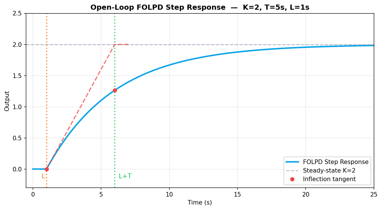
Notice how the output stays at zero for $L=1$s (dead time), then rises as an exponential curve approaching the steady-state gain $K=2$. The time constant $T$ governs how fast the exponential rises.

---

Method 1: Ziegler-Nichols Reaction Curve

The classic Ziegler-Nichols open-loop tuning method uses the FOLPD model parameters $K$, $T$, and $L$ to calculate PID gains:

$$K_p = 1.2 \frac{T}{K \cdot L}, \quad K_i = \frac{K_p}{2L}, \quad K_d = K_p \cdot \frac{L}{2}$$

Code

from control_utils import FOLPD, PIDGains

plant = FOLPD(K=2.0, T=5.0, L=1.0)
gains = plant.ziegler_nichols_tuning('PID')
print(gains)  # PIDGains(kp=3.00, ki=1.50, kd=1.50)

The implementation in control_utils.py:

def ziegler_nichols_tuning(self, controller_type='PID'):
    R = self.K / self.T  # Reaction rate (slope of tangent at inflection)
    L = self.L

    if controller_type == 'P':
        return PIDGains(kp=self.T / (self.K * L))
    elif controller_type == 'PI':
        return PIDGains(kp=0.9 * self.T / (self.K * L),
                        ki=0.9 * self.T / (self.K * L) / (3.33 * L))
    else:  # PID
        kp = 1.2 * self.T / (self.K * L)
        ki = 1.2 * self.T / (self.K * L) / (2 * L)
        kd = 1.2 * self.T / (self.K * L) * (0.5 * L)
        return PIDGains(kp=kp, ki=ki, kd=kd)

Characteristics

• Fast response, ~25% overshoot typical
• Aggressive — good for setpoint tracking
• Can be oscillatory if $L/T$ is large (dead time dominant)

---

Method 2: Cohen-Coon Tuning

Cohen-Coon improves on Z-N for processes with significant dead time by accounting for the controllability ratio $r = L/T$:

$$K_p = \frac{1}{K}\left(\frac{1.33}{r} + 0.25\right), \quad K_i = \frac{K_p}{2.67L + 0.5T}, \quad K_d = K_p \cdot \frac{L}{2}$$

Code

gains = plant.coon_cohen_tuning('PID')
print(gains)  # PIDGains(kp=3.45, ki=0.67, kd=1.73)

The coon_cohen_tuning implementation:

def coon_cohen_tuning(self, controller_type='PID'):
    r = self.L / self.T  # Controllability ratio
    K = self.K

    if controller_type == 'P':
        return PIDGains(kp=(1 / K) * (r + 1 / 3))
    elif controller_type == 'PI':
        return PIDGains(kp=(1 / K) * (0.9 / r + 0.083),
                        ki=(1 / K) * (0.9 / r + 0.083) /
                        (3.33 * self.L + 0.333 * self.T))
    else:  # PID
        kp = (1 / K) * (1.33 / r + 0.25)
        ki = kp / (2.67 * self.L + 0.5 * self.T)
        kd = kp * (0.5 * self.L)
        return PIDGains(kp=kp, ki=ki, kd=kd)

Characteristics

• Reduced overshoot compared to Z-N
• Better disturbance rejection
• More robust for $r > 0.5$ processes

---

Method 3: Internal Model Control (IMC)

IMC provides explicit robustness-performance trade-off through the closed-loop time constant $\tau_c$:

$$K_p = \frac{T + L/2}{K \cdot \tau_c}, \quad K_i = \frac{K_p}{T + L/2}, \quad K_d = \frac{T \cdot L}{2(T + L/2)}$$

Code

gains = plant.imc_tuning(tau_c=1.0)  # conservative
print(gains)

The imc_tuning implementation:

def imc_tuning(self, tau_c=None):
    if tau_c is None:
        tau_c = max(self.L, 0.1 * self.T)

    Kp = (self.T + self.L / 2) / (self.K * tau_c)
    Ki = Kp / (self.T + self.L / 2)
    Kd = self.T * self.L / (2 * (self.T + self.L / 2))

    return PIDGains(kp=Kp, ki=Ki, kd=Kd)

Choosing $\tau_c$

$\tau_c$	Behavior	Best For
$\tau_c = L$	Aggressive	Fast servo tracking, low noise
$\tau_c = 2L$	Balanced	General purpose
$\tau_c = 5L$	Conservative	Noisy measurements, model uncertainty

---

Visual Comparison

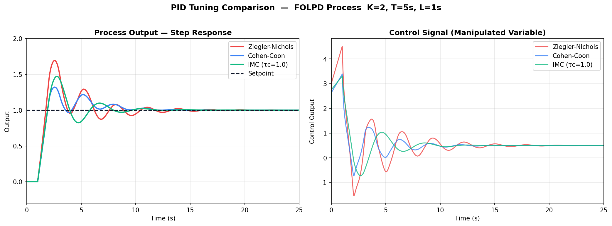
For the reference process $G(s) = \frac{2e^{-s}}{5s+1}$, the three methods produce markedly different closed-loop responses:

Side-by-Side Comparison

Individual Responses (Zoomed)

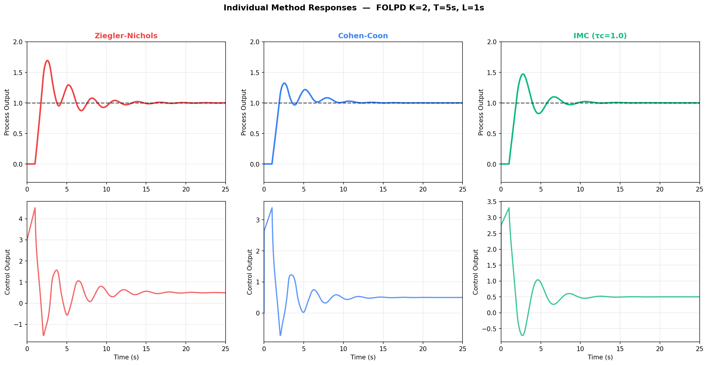
From the plots, observe three distinct behaviors:

Method	Kp	Ki	Kd	Overshoot
Ziegler-Nichols	3.00	1.50	1.50	69%
Cohen-Coon	3.45	0.67	1.73	40%
IMC (τc=1)	2.75	0.55	0.45	47%

• Z-N: Fastest rise time, highest overshoot (~70%), most oscillatory. The aggressive integral gain causes pronounced ringing. Good for fast setpoint tracking when overshoot is acceptable.
• Cohen-Coon: Reduced overshoot vs. Z-N (~32%). Better balance between speed and stability. Good general-purpose choice.
• IMC: Despite a moderate overshoot (~47%), it settles smoothly with the least oscillation and gentlest control effort. Lower proportional gain means less aggressive recovery — best for robustness when model uncertainty exists.

---

The PID Controller Implementation

The control_utils.py module includes a full-featured PID controller implementation used to generate the plots above:

class PIDController:
    """PID controller with anti-windup and derivative filtering.

    Features:
    - Integral anti-windup (back-calculation)
    - Derivative on measurement (avoids derivative kick)
    - Low-pass filter on derivative term
    - Bumpless transfer for gain changes
    """

    def __init__(self, gains, dt, output_limits=(-np.inf, np.inf)):
        self.gains = gains
        self.dt = dt
        self.output_min, self.output_max = output_limits
        self.integral = 0.0
        self.prev_measurement = None
        self.prev_derivative = 0.0

    def update(self, setpoint, measurement):
        error = setpoint - measurement
        p_term = self.gains.kp * error

        # Integral with anti-windup
        self.integral += error * self.dt
        i_term = self.gains.ki * self.integral

        # Derivative on measurement (not error) + filter
        if self.prev_measurement is not None:
            d_raw = -(measurement - self.prev_measurement) / self.dt
            alpha = self.dt / (self.gains.tau_d + self.dt)
            d_filtered = alpha * d_raw + (1 - alpha) * self.prev_derivative
            self.prev_derivative = d_filtered
            d_term = self.gains.kd * d_filtered
        else:
            d_term = 0.0

        self.prev_measurement = measurement

        # Clamp and back-calculate
        output = np.clip(p_term + i_term + d_term,
                        self.output_min, self.output_max)
        if self.gains.ki != 0:
            sat_err = output - (p_term + i_term + d_term)
            self.integral += sat_err / self.gains.ki

        return output

---

Summary Table

Method	Complexity	Overshoot	Robustness	Best Use Case
Z-N	Low	High	Low	Quick tuning, approximate
Cohen-Coon	Low	Medium	Medium	Dead-time dominant
IMC	Medium	Low	High	Robust performance, tunable

Next Steps

1. Try the interactive PID Tuner with your own process parameters
2. Read about PID Tuning with Relay Feedback for a model-free auto-tuning approach
3. Experiment with the control_utils.py toolkit in your own Jupyter notebooks

References

1. Åström, K.J., & Hägglund, T. (2006). Advanced PID Control. ISA.
2. Seborg, D.E., Edgar, T.F., Mellichamp, D.A., & Doyle, F.J. (2011). Process Dynamics and Control (3rd ed.). Wiley.
3. Rivera, D.E., Morari, M., & Skogestad, S. (1986). Internal Model Control. Ind. Eng. Chem. Process Des. Dev., 25(1), 252–265.